Data Manipulation In R
Introduction
We will use the MEPS dataset for the purposes of this tutorial. The MEPS dataset is a population dataset of medical expenditure data in the United States.
data <- read.csv(url("https://laurencipriano.github.io/IveyBusinessStatistics/Datasets/mepsData.csv"), header = TRUE)Making new rows and columns
We can use rbind and cbind to add new rows
and columns respectively. They must have the same structure in order to
work.
sample_row = data[1337, ] # Picking a random row for the example

data_subset = rbind(data, sample_row)
nrow(data)
> [1] 30461nrow(data_subset)> [1] 30462An easier way to make new columns when working with data.frames is by
using the $.
data2 = data # Keep our original dataset untouched.
data2$newColumn = 1 # Fill the column entirely with 1's
summary(data2$newColumn)
> Min. 1st Qu. Median Mean 3rd Qu. Max.
> 1 1 1 1 1 1Taking Slices of Data
Often you will find that you require only portions of a dataset.
The most basic method is to directly pass the row or column number or name.
data_subset = data[ , c("Person_ID", "Age", "Sex")] # Keep these columns
summary(data_subset)> Person_ID Age Sex
> Min. :2290001101 Min. : 0.0 Min. :0.000
> 1st Qu.:2294946102 1st Qu.:18.0 1st Qu.:0.000
> Median :2320170102 Median :38.0 Median :0.000
> Mean :2310116491 Mean :39.1 Mean :0.479
> 3rd Qu.:2325003103 3rd Qu.:59.0 3rd Qu.:1.000
> Max. :2329687103 Max. :85.0 Max. :1.000
> NA's :375data_subset = data[1:10000, ] # Keeping the first 10000 rows
summary(data_subset)> Observation Person_ID FluVaccination Age
> Min. : 1 Min. :2290001101 Min. :0.000 Min. : 0.0
> 1st Qu.: 2501 1st Qu.:2291636102 1st Qu.:0.000 1st Qu.:17.0
> Median : 5000 Median :2293230152 Median :0.000 Median :38.0
> Mean : 5000 Mean :2293240888 Mean :0.415 Mean :38.5
> 3rd Qu.: 7500 3rd Qu.:2294875102 3rd Qu.:1.000 3rd Qu.:58.0
> Max. :10000 Max. :2296506103 Max. :1.000 Max. :85.0
> NA's :3749 NA's :98
> Sex RaceEthnicity HealthInsurance NotAffordHealthCare
> Min. :0.00 Min. :1.0 Min. :1.0 Min. :0.0000
> 1st Qu.:0.00 1st Qu.:1.0 1st Qu.:1.0 1st Qu.:0.0000
> Median :0.00 Median :2.0 Median :1.0 Median :0.0000
> Mean :0.48 Mean :2.1 Mean :1.5 Mean :0.0479
> 3rd Qu.:1.00 3rd Qu.:2.0 3rd Qu.:2.0 3rd Qu.:0.0000
> Max. :1.00 Max. :5.0 Max. :3.0 Max. :1.0000
> NA's :176
> FamIncome_Continuous MentalHealth FamIncome_Categorical
> Min. : 0 Min. :1.00 Min. :1.00
> 1st Qu.: 26000 1st Qu.:1.00 1st Qu.:3.00
> Median : 54906 Median :2.00 Median :4.00
> Mean : 73092 Mean :2.07 Mean :3.51
> 3rd Qu.:100000 3rd Qu.:3.00 3rd Qu.:5.00
> Max. :507855 Max. :5.00 Max. :5.00
> NA's :4 NA's :167
> FamIncome_PercentPoverty HealthStatus HaveProvider CensusRegion
> Min. : 0 Min. :1.00 Min. :0.000 Min. :1.00
> 1st Qu.: 132 1st Qu.:1.00 1st Qu.:1.000 1st Qu.:2.00
> Median : 262 Median :2.00 Median :1.000 Median :3.00
> Mean : 352 Mean :2.23 Mean :0.775 Mean :2.72
> 3rd Qu.: 479 3rd Qu.:3.00 3rd Qu.:1.000 3rd Qu.:3.00
> Max. :3020 Max. :5.00 Max. :1.000 Max. :4.00
> NA's :4 NA's :164 NA's :439 NA's :98
> TotalHealthExpenditure HasHypertension HasDiabetes BMI
> Min. : 0 Min. :0.00 Min. :0.0000 Min. : 0.1
> 1st Qu.: 186 1st Qu.:0.00 1st Qu.:0.0000 1st Qu.:23.6
> Median : 1062 Median :0.00 Median :0.0000 Median :27.4
> Mean : 6120 Mean :0.35 Mean :0.0959 Mean :28.2
> 3rd Qu.: 4674 3rd Qu.:1.00 3rd Qu.:0.0000 3rd Qu.:32.1
> Max. :807611 Max. :1.00 Max. :1.0000 Max. :71.1
> NA's :2674 NA's :94 NA's :4072We will want to do more complex slices as our data may contain outliers, or you are investigating specific individuals.
Let’s take a look at some useful functions.
Subset
hist(data$FamIncome_Continuous)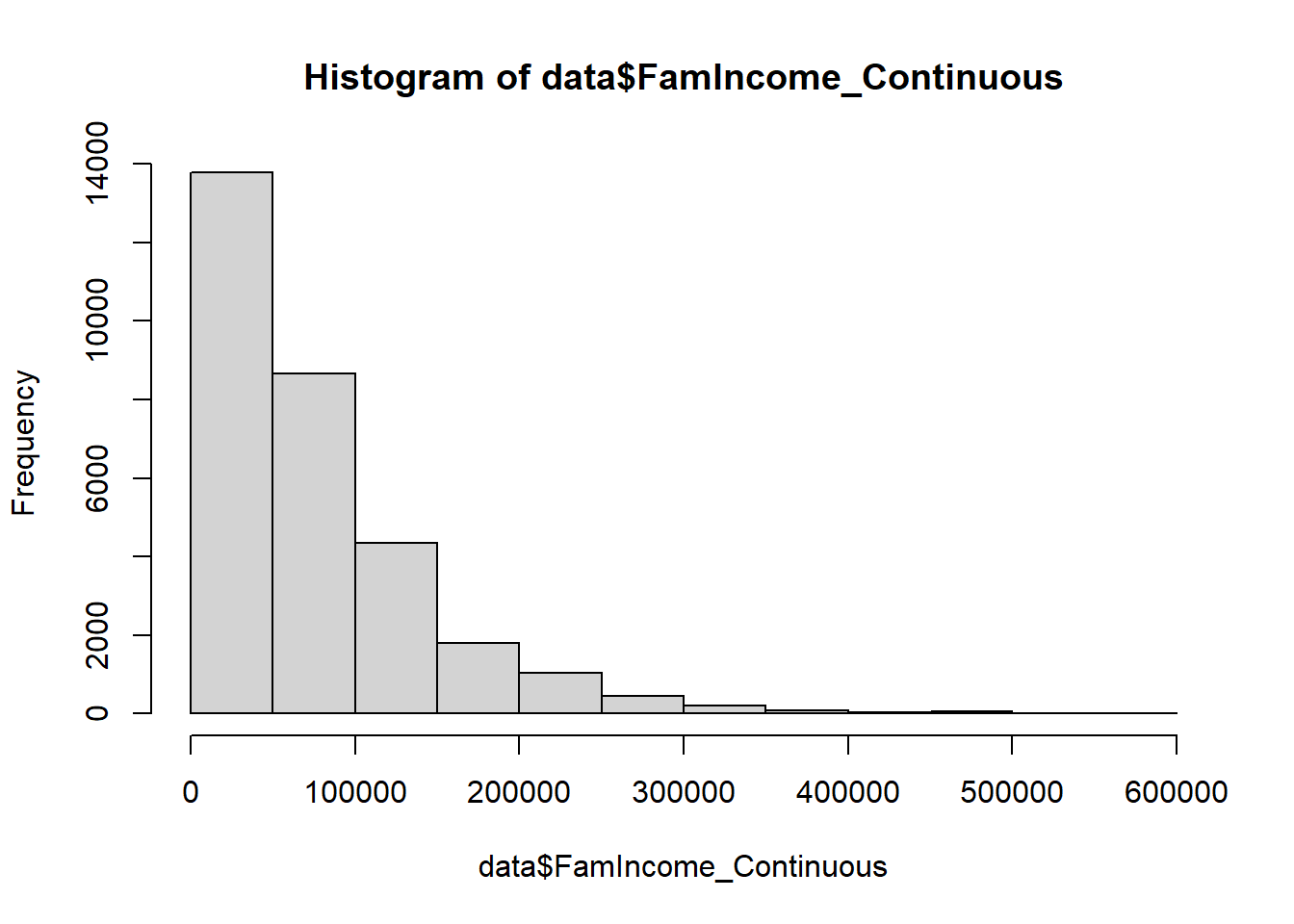
As you can see, the majority of data points lie below $300,000. Let’s
take a clearer look at those individuals by taking advantage of the
subset function.
data_subset = subset(data, FamIncome_Continuous<300000)
hist(data_subset$FamIncome_Continuous)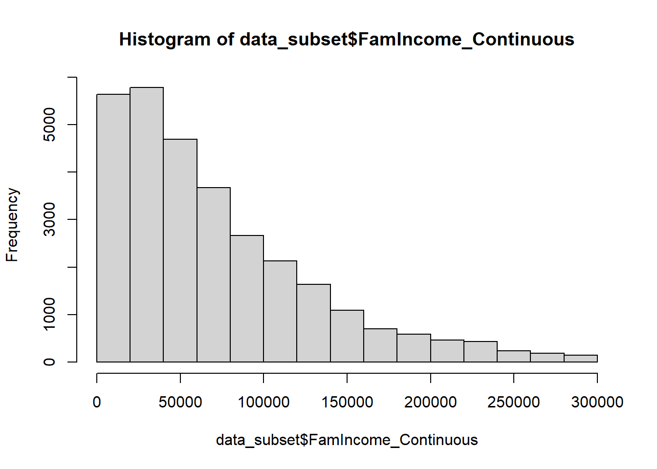
The dataset now only contains individuals below our target income. We can investigate the impact this has on the entire dataset below.
summary(data$FamIncome_Continuous)
> Min. 1st Qu. Median Mean 3rd Qu. Max. NA's
> 0 26895 56532 75267 103882 583219 14
summary(data_subset$FamIncome_Continuous)
> Min. 1st Qu. Median Mean 3rd Qu. Max.
> 0 26370 55538 71651 100916 299406The
subsetfunction can be used on vectors, matrices and data frames!
Which
For even more complex slices of data, the which function
comes in handy. It works a little differently…the which
function provides indices where our logic is true, so we have to pass
the which function as an input for the rows to keep.
Let’s investigate individuals with Normal BMI classification (18.5-25) who have diabetes.
# Will provide a vector telling us which indices are TRUE
index = which(data$HasDiabetes==1 & #Combine statements with &
data$BMI>18.5 &
data$BMI<25)
head(index) #See the first six elements of index> [1] 300 444 446 511 605 681data_subset = data[index, ] # We leave the column input blank to include all columnssummary(data_subset$HasDiabetes)
>    Min. 1st Qu.  Median    Mean 3rd Qu.    Max.
>       1       1       1       1       1       1
summary(data_subset$BMI)
> Min. 1st Qu. Median Mean 3rd Qu. Max.
> 18.6 21.6 23.1 22.8 24.2 24.9Removing NA’s
We may be investigating the impact of hypertension. As you can see
below, the HasHypertension column has some missing
entries.
summary(data$HasHypertension)> Min. 1st Qu. Median Mean 3rd Qu. Max. NA's
> 0.000 0.000 0.000 0.348 1.000 1.000 7725The is.na function tests whether a variable contains
NA.
is.na(1)
> [1] FALSE
is.na(NA)
> [1] TRUE
is.na(c(1,2,3,NA))
> [1] FALSE FALSE FALSE  TRUE
We can use the is.na function combined with either of
our methods above.
data_subset = subset(data, is.na(HasHypertension)==0)
# or
index = which(is.na(data$HasHypertension)==0)
data_subset = data[index, ]
The data now contains only rows where hypertension is not missing.
summary(data$HasHypertension)> Min. 1st Qu. Median Mean 3rd Qu. Max. NA's
> 0.000 0.000 0.000 0.348 1.000 1.000 7725summary(data_subset$HasHypertension) > Min. 1st Qu. Median Mean 3rd Qu. Max.
> 0.000 0.000 0.000 0.348 1.000 1.000Replacing Missing Data
We can take this one step further. Rather than simply removing missing data, we can replace is with the population average. Notice BMI has many missing entries.
summary(data$BMI)> Min. 1st Qu. Median Mean 3rd Qu. Max. NA's
> 0.1 23.7 27.3 28.2 31.9 71.1 12209Let’s replace it with the average BMI from the remaining population.
# Keeping our original dataset untouched
data2 = data

# First find the indices where BMI is missing
index = which(is.na(data2$BMI)==1)

# Replace the BMI at those indices
data2[index, "BMI"] = mean(data2$BMI, na.rm = TRUE)

summary(data2$BMI)
> Min. 1st Qu. Median Mean 3rd Qu. Max.
> 0.1 26.1 28.2 28.2 28.5 71.1We can use any method to replace the missing data, try using the
medianandmodefunctions on your own!
Merge
If we try to use rbind to combine datasets we may get
some unwanted behaviour.
data_subset_diab = subset(data, HasDiabetes==1)
data_subset_hyper = subset(data, HasHypertension==1)

data_subset = rbind(data_subset_diab, data_subset_hyper) # Use rbind to directly combine the tables by row

nrow(unique(data_subset)) # Number of unique observations
> [1] 8633
nrow(data_subset) # Total Observations
> [1] 10805
As you can see, there are more total observations than unique
observations. We are double counting some observations as there are
people with both diabetes and hypertension. This is where the
merge function comes in handy.
data_subset = merge(data_subset_diab, data_subset_hyper, by = "Person_ID", all = TRUE, sort = TRUE)

nrow(data_subset)
> [1] 8633The all parameter tells the function to keep any
observation that does not have a matching ID, achieving the behaviour we
desire.
Remember to check out the help page for any function (using
help(merge)), they have even more useful information!
Converting Continuous to Categorical (Factors)
Sometimes we may want to investigate our variables as categories. We can convert columns in our table easily. Let’s convert our continuous BMI variable into commonly used classifications. We will use the dataset where we replaced missing values with mean BMI.
BMICategories = c("Underweight", "Normal Weight", "Overweight", "Obese")

# Initializing column with zeros
data2$BMICategory = 0
We must first initialize our categories with simple integers, we will use 1-4 to represent our four categories. The logic within the square brackets tells our data.frame to update only the rows where the statement is true.
# Underweight
data2$BMICategory[ data2$BMI<18.5 ] = 1
# Normal Weight
data2$BMICategory[ data2$BMI>=18.5 & data2$BMI<25 ] = 2
# Overweight
data2$BMICategory[ data2$BMI>=25 & data2$BMI<30 ] = 3
# Obese
data2$BMICategory[ data2$BMI>=30 ] = 4
Next we can apply labels and convert the column to a factor, making it easier to read. The levels and labels parameters are telling our factor to associate the values of 1-4 with the labels we made earlier.
data2$BMICategory = factor(data2$BMICategory,
                           levels = c(1,2,3,4),
                           labels = BMICategories)
We can see now our new column now.
summary(data2$BMICategory)> Underweight Normal Weight Overweight Obese
> 709 5362 18158 6232Making a Binary from Continuous
Perhaps we would like to do something even simpler. We can make a new
binary column called HealthyWeight.
# Create new column as FALSE
data2$HealthyWeight = FALSE

# Convert individuals to TRUE
data2$HealthyWeight[ data2$BMI>=18.5 & data2$BMI<25 ] = TRUE

summary(data2$HealthyWeight)
> Mode FALSE TRUE
> logical 25099 5362Notice we could also use our new BMICategory column!
# Set column as FALSE
data2$HealthyWeight = FALSE

# Convert individuals to TRUE
data2$HealthyWeight[ data2$BMICategory=="Normal Weight" ] = TRUE

summary(data2$HealthyWeight)
> Mode FALSE TRUE
> logical 25099 5362